library(tidycensus)
library(tigris)
library(sf)
library(arcgislayers)
library(tidyverse)
library(patchwork)
options(tigris_use_cache = T)Quantifying the local impact of wildfire on demographic factors
Introduction
Wildland fire and its relationship with land management is a contentious topic, particularly in a post-Industrial-Revolution climate. Since the 1935 advent of the Forest Service’s “ten-A.M. policy,” fire suppression has been the standard in land management: protection of economic interests including timber stands (for logging) and grasslands (for grazing) has been priority one (Westover 2023). However, this philosophy has shifted slowly as the ecological benefits of wildland fire have shown themselves in various ecosystems – lodgepole pines need the heat to open their cones, wild lupine needs fire to clear mid-canopy plants that outcompete it for sunlight, and the clearing of ladder fuels prevent future catastrophic crowning fires. Today, the Forest Service has a new position on wildland fire – when possible, let it burn.
However, this is often impossible when fires burn into areas occupied by humans; protection of life, property, and prosperity becomes priority one. The groups most vulnerable to wildfire impacts are those who are marginalized in spaces across America: Davies et al. (2018) found that census tracts with majority Black, Hispanic, and Native American populations were about twice as vulnerable to wildfire impacts when compared to other census tracts.
Goals
My goals for this project are to:
Facilitate easier gathering of data related to wildland fire
Investigate the historic relationships between wildland fire and people by incorporating Census demographic data
Improve my functional and literate programming skills in R
Hopefully, anyone who is affected by historic wildfires would find this research useful; whether that be individuals, jurisdictions, land stewards, or conservationists. I don’t plan on computing an index; doing so would require a discussion of what a “negative social characteristic” is. The output object will contain the change in social variables between pre- and post-event years, but a single “impact index” will not be calculated.
Data
There are two types of data I’m planning to use as proofs of concept for this project. The first is historic federal interagency wildland fire data, which is maintained by the National Interagency Fire Center (NIFC) and distributed via ArcGIS Online products including hosted feature layers and an Esri Hub site. The bulk of the data can be accessed from within R by using the arcgislayers package to query the NIFC ArcGIS REST server (link).
In particular, the Interagency Fire Perimeter History layer will be used to access historic wildland fire perimeters. The earliest recorded fire in this dataset started in 708 A.D., determined by carbon dating – however, a more realistic subset of wildland fires will be selected based on overlapping temporal ranges with Census data. Full documentation and metadata for the layer can be found via its NIFC ArcGIS Hub page, which provides a more readable interface for traditional GIS users.
The second data repository I’ll use to support my work is the Census Bureau’s ACS 5-year estimates, which contain annual estimates of demographic information from 2009 onward. ACS information will be accessed using tidycensus and tigris, which will allow for spatial operations including spatial filtering and population-weighted interpolation. Information regarding ACS data can be found at the Census Bureau’s ACS homepage.
The more unfamiliar and nonstandard of these sources is likely the NIFC perimeter data. It can be collected in the field, drawn in a desktop GIS, or derived from imagery, depending on the size of the fire, terrain, and available staffing, among other considerations. Luckily, it contains a field describing the method of collection for each fire; this can be used to determine which perimeters are more accurate for our uses. In addition, each row contains information corresponding to the responsible agency, event names, and unique event IDs.
As all of these sources are maintained and distributed by the federal government, they have generally permissive licensing:
- NIFC: https://data-nifc.opendata.arcgis.com/datasets/nifc::interagencyfireperimeterhistory-all-years-view/about (click on “View license details” on the right side of the page)
- Census Bureau API: https://www.census.gov/data/developers/about/terms-of-service.html
My usage of these data sources is without warranty, and my work is not endorsed nor certified by either the U.S. Census Bureau or the National Interagency Fire Center.
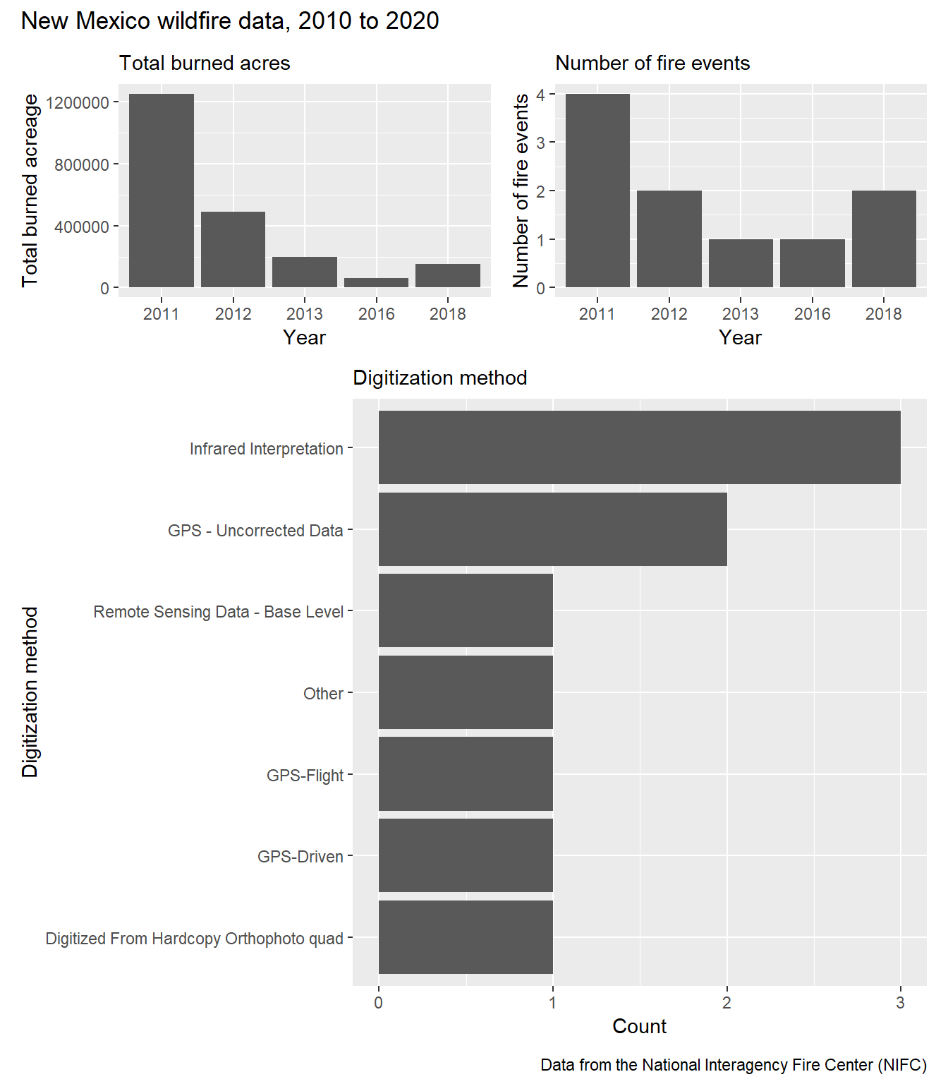
As a demonstration, I’ll use the ten largest New Mexican wildfires in the NIFC historic perimeter database between 2010 and 2020.
# Example of tigris:
nm <- tigris::states() |>
dplyr::filter(STUSPS == "NM") |>
st_as_sfc()
# Example of arcgislayers:
nm_fires <- arcgislayers::arc_read(r"(https://services3.arcgis.com/T4QMspbfLg3qTGWY/ArcGIS/rest/services/InterAgencyFirePerimeterHistory_All_Years_View/FeatureServer/0)",
where = "FIRE_YEAR BETWEEN 2010 AND 2020",
filter_geom = nm
) |>
st_make_valid(geos_method = "valid_linework") |>
distinct(toupper(INCIDENT), .keep_all = T) |>
slice_max(
order_by = Shape__Area,
n = 10
) |>
select(-`toupper(INCIDENT)`) |>
mutate(COMMENTS = str_trunc(COMMENTS, 35))
mapview::mapview(nm_fires)
Planned approach
My goal is to create a function which will show the impact of nonspecific disasters on social and economic variables by extracting Census data via tidycensus. The Census Bureau has released OnTheMap for Emergency Management, which gathers relevant social variables for ongoing events. However, I don’t believe there exists a version which shows the values before and after historic events.
My approach is to allow a user to input an sf object and a year, and get back ACS estimates on variables including race/ethnicity, total population, and household income, by default. The variables option will allow a user to input their own variables, in tidycensus syntax, which will be summarized accordingly. By naming the variables in the variables option, the user can specify the summarization operation to be used: for example, mean_household_size is aggregated using mean(), and median_household_income is aggregated using median(). Variable names that do not follow these string patterns will be treated as extensive, and will be aggregated using sum().
The exciting thing about this approach is that a user can input a novel sf object with a field containing a year, and compute the demographics for all tracts it intersected with for a given range before and after that year. So, a polygon detailing a disaster could be drawn using mapedit, for example, and its effect on the surrounding demographics would be computed.
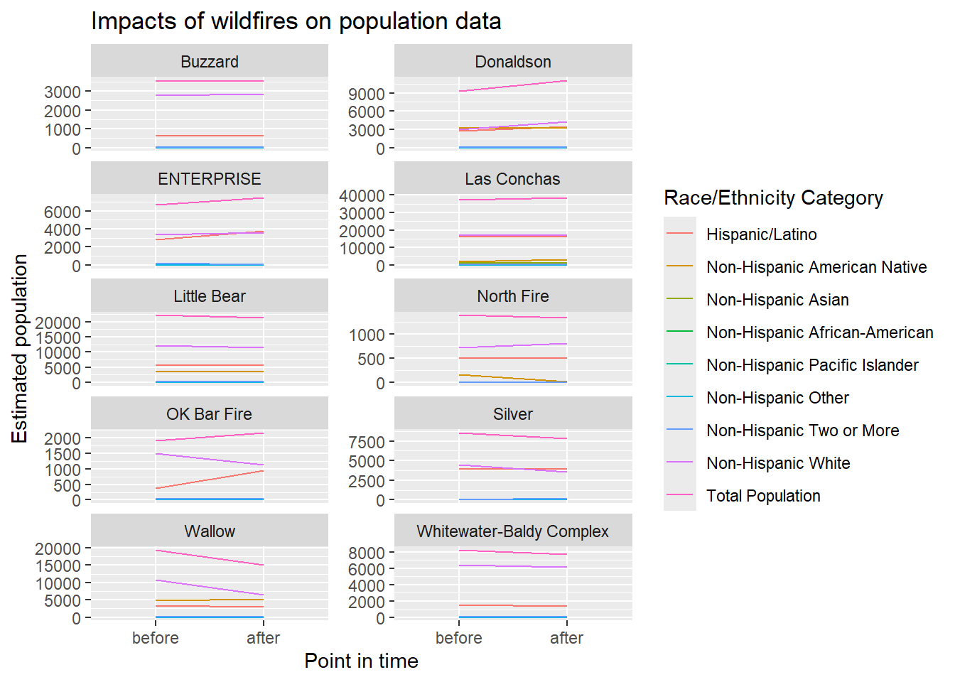
Using the nm_fires object created earlier, here is a brief demonstration of how the function works. The output object is an sf object, which contains all of the original incident fields – however, to the right side of this table, the requested demographic info is appended.
When output = "tidy" (the default), differences are not computed and the information is returned in a long-format table, with a row per point in time (e.g., before and after the event) and per variable. When output = "wide" is specified, the absolute differences between the two time points are computed, and the original variables are not returned to aid with GIS and cartography.
nm_fires_impact <- get_incident_impacts(
data = nm_fires,
id_col = OBJECTID,
year = FIRE_YEAR
)ggplot(filter(nm_fires_impact, str_starts(variable, "pop"))) +
geom_line(aes(x = fct_rev(pt_in_time), y = computed, group = variable, color = variable)) +
xlab("Point in time") +
ylab("Estimated population") +
labs(title = "Impacts of wildfires on population data") +
scale_color_discrete("Race/Ethnicity Category", labels = c(
"Hispanic/Latino",
"Non-Hispanic American Native",
"Non-Hispanic Asian",
"Non-Hispanic African-American",
"Non-Hispanic Pacific Islander",
"Non-Hispanic Other",
"Non-Hispanic Two or More",
"Non-Hispanic White",
"Total Population"
)) +
facet_wrap(~INCIDENT, scales = "free_y", nrow = 5, ncol = 2)
nm_fires_impact_wide <- get_incident_impacts(
data = nm_fires,
id_col = OBJECTID,
year = FIRE_YEAR,
output = "wide"
)mapview::mapview(nm_fires_impact_wide,
zcol = "median_hhi"
)A presentation with more details, given in class, can be found here.